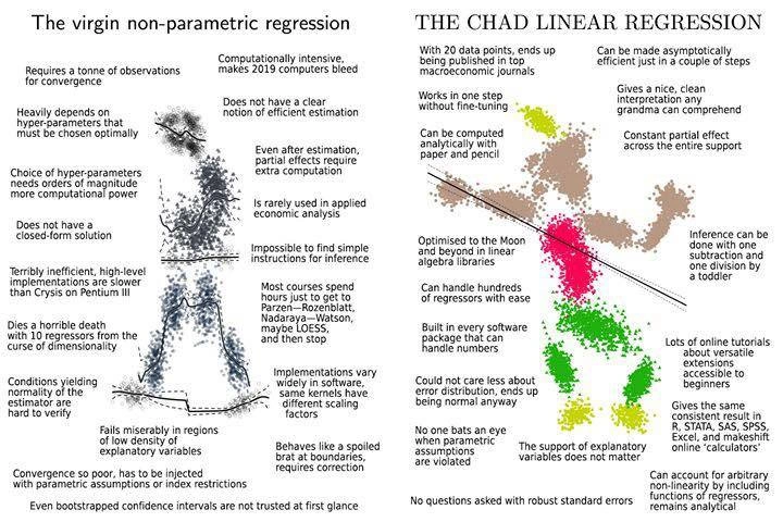
Virgin Non-Parametric Regression vs Chad Linear Regression Comparison

Level 1: Hammer It Home

Imagine you want to hang a picture on your wall. You’ve got two friends offering to help. The first friend shows up with this over-the-top contraption – it’s like a wacky machine with gears, sensors, and a laser guide, all designed to hammer a nail precisely. But to use it, you have to set a bunch of dials just right, it takes forever to calibrate, and if the wall is a tiny bit different from what it expects (say the wood is harder or the spot is a little out of range), the machine just sputters and fails. This is like the non-parametric regression in the meme: super fancy and theoretically cool, but needs a lot of attention and still might not work outside its comfort zone.

Now the second friend just comes in, picks up a simple hammer, and bam – knocks the nail into the wall in one go. Picture hanging accomplished. That’s the linear regression: the trusty hammer of data analysis. It’s not fancy or new, but boy does it get the job done with minimal fuss. No special setup, no delicate adjustments, it just works everywhere you’d reasonably need it.

The meme is basically saying that sometimes, trying to be too fancy is like using that over-engineered nail robot (frustrating and overkill), whereas using a straightforward tool like the hammer can be a total Chad move – confident, effective, and done before you know it. In everyday terms: sometimes the simplest solution really is the best solution.

Level 2: Curves vs Straight Lines

Let’s break this down in simpler terms and define some of the jargon. We have two competing approaches to statistical modeling here: one that draws a single straight line through the data, and one that tries to draw a curvy, flexible line fitting the data points closely. The straight-line approach is linear regression, often specifically Ordinary Least Squares (OLS). The curvy approach is a type of non-parametric regression (examples include methods like kernel regression or LOESS smoothing). The meme humorously compares these two like a weak “virgin” and a strong “Chad”.

• Linear Regression (OLS): This is the simplest kind of regression analysis. Imagine you have a scatter plot of points (each point might represent, say, a city’s population on the x-axis and its COVID cases on the y-axis, or any cause-and-effect pair). Linear regression draws the best-fit straight line through those points. “Best-fit” usually means it minimizes the sum of squared vertical distances from the points to the line (that’s the “least squares” part). With OLS, you end up with a formula like Y = β0 + β1 * X1 + β2 * X2 + ... + βp * Xp (for multiple factors, but if there’s just one X, it’s Y = β0 + β1 * X). The β coefficients are numbers the method finds for you (e.g., β1 is the slope). Once you have those, you can plug in an X value and get a predicted Y. Importantly, OLS has a closed-form solution – basically, there’s a direct mathematical formula to compute all the βs from your data (no trial-and-error needed). Because of that, running linear regression is super easy and fast with any stats software or even a few lines of code. Also, interpreting the results is straightforward: β1 = 5 means “if X increases by 1, Y tends to increase by 5”. This simplicity and clarity is why we say OLS “gives a nice, clean interpretation” and why it’s taught early in DataScience courses. It’s built into every major analysis tool – Excel, R, Python’s sklearn, you name it – just supply your data and you get the line. Another thing: linear regression doesn’t need you to guess any hyperparameters. There’s no knob to turn for “how straight should the line be” – it’s always a straight line by definition 😄. At most, you might decide to transform some data or add an interaction term, but those are modeling choices, not mysterious tuning parameters.

• Non-parametric Regression: This is a fancier approach where we don’t assume the relationship is a straight line (or any fixed formula). Instead, we let the data points dictate the shape of the curve. One simple example is LOESS (Locally Estimated Scatterplot Smoothing), which basically draws a smooth curve through the cloud by stitching together lots of tiny straight lines or low-degree polynomials that fit local neighborhoods of the data. Another example is kernel regression (like the Nadaraya–Watson method mentioned), which predicts a new Y by looking at nearby data points’ Ys and averaging them, with closer points given more weight (the weights come from a kernel function, which is just a fancy peaked curve, kind of like a bump that says “how much influence does a point have based on its distance from the query”). In non-parametric regression, you don’t say “it must be a line” or “it must be a quadratic” – you let it be whatever shape fits. Sounds great, right? The catch is that because you’re not restricting the shape, you often need a lot more data to get a reliable curve. If you only have a few points, a flexible method might draw some crazy zigzag just to go exactly through those points (that’s effectively overfitting – fitting the noise). With more points, the hope is the zigzagging evens out into a sensible smooth curve. The meme mentions “requires a ton of observations for convergence” – exactly this idea that these methods need lots and lots of data to pin down the underlying pattern reliably.

• Hyperparameters: This word appears several times in the virgin side’s complaints. A hyperparameter is like a setting for the model that you, the user, have to decide (often by trial, intuition, or extra procedures), rather than the model learning it from the data directly. For example, in a kernel_regression, a crucial hyperparameter is the bandwidth (usually denoted h). Bandwidth roughly means “how wide is the neighborhood I look at when averaging points.” A small bandwidth means I only consider very close points (result: a very wiggly, sensitive curve that can capture fine details but also noise – high variance risk). A large bandwidth means I consider faraway points too (result: a smoother, more stable curve but potentially missing local quirks – high bias risk). Choosing the right bandwidth is an art: too small and you overfit, too large and you oversimplify. And there’s no simple formula for the best bandwidth – you typically have to use methods like cross-validation (try various values and see which predicts best on held-out data). That’s why the meme says “choice of hyper-parameters needs orders of magnitude more computation time”: you might literally run the whole regression many times for different hyperparameter guesses to find a decent one. In MachineLearning more broadly, hyperparameters include things like the number of layers in a neural network, the depth of a decision tree, the learning rate in gradient descent, etc. The hyperparameter_hell phrase is a jokey way to describe the frustration of tuning these – it can feel like an endless dark tunnel of tests and tweaks. OLS, by contrast, has basically no hyperparameters to tune (besides maybe deciding which variables to include, but that’s more about model selection than algorithm settings). So you run it once and you’re done – no hellish search.

• Closed-form solution: This means we have a direct mathematical answer. For OLS linear regression, there is a formula (as mentioned above) to compute the best-fit line from the data in one go. Non-parametric regression doesn’t have that luxury. There isn’t a simple formula to get “the curve” – you have to compute it point by point or via iterative procedures. Think of it like this: OLS is like solving a quadratic equation with the formula $x = [-b \pm \sqrt{b^2-4ac}]/(2a)$ – straightforward. Non-parametric is like trying to solve something without a formula, where you might need to resort to numerical approximations or just crunching through the data.

• Support of the data: The support just means the range of values your input variables cover. For example, if all your X data runs from 0 to 100, that’s the support of X in your sample. If you ask the model to predict for X = 150 (which is outside that support), a linear_regression will extrapolate (it will plug 150 into the line equation and give a result, which could be very iffy, but it does produce a number). A non_parametric_regression typically can’t extrapolate confidently because, say in a kernel method, X=150 is too far from any known data points to have meaningful weights – the predictions become essentially a guess. Often, non-parametric implementations will either not let you predict beyond the range or will return something like the prediction tends towards the overall mean. That’s why the meme jokes it “dies a horrible death” outside support – it’s dramatizing that these methods are really meant for interpolation (filling in between known data points), not extrapolation (going beyond). Linear models are much more cavalier: they’ll give you a straight-line answer whether or not it’s sensible – hence “The support … does not matter” on the Chad side (though as users we should be careful, the meme is just simplifying things for the joke).

• Efficiency and implementation differences: The meme contrasts “Terribly inefficient, high-level implementations are slower than Crysis on Pentium III” with “Optimized to the Moon and beyond in linear algebra libraries”. In simpler words, this is about how easy it is to compute these things with standard tools. Linear regression can use very efficient matrix operations under the hood (leveraging low-level, fast languages like C, Fortran, or optimized math libraries that make use of your CPU/GPU). Non-parametric methods (like those written in, say, pure Python or R loops for each prediction) might be much slower because they’re doing a lot more work and possibly not leveraging those low-level optimizations. Crysis on a Pentium III was basically a meme itself: Can it run Crysis? was a way of asking if a computer was powerful back in late 2000s, and a Pentium III is an old processor – a combo implying something is comically slow or demanding. So they’re humorously saying some implementations of non-parametric regression are brutally slow for what they do, whereas linear regression is lightning-fast thanks to years of optimization. For a beginner, the takeaway is: simple methods tend to be not just easier to use but also easier for computers to run quickly, because they involve simpler math and leverage existing efficient algorithms. Complex, flexible methods might involve more complex calculations that aren’t as optimized, or require writing more code that can be slower if not done carefully.

• Partial effects: This term might be new unless you’ve taken some economics or advanced stats classes. It means the effect of one input variable on the output, holding others constant – basically the slope or rate of change. In a linear model, it’s literally the coefficient (β) for that variable, and it’s the same no matter where you are. For example, if β_age = 2 in a wage regression, it means “each additional year of age is associated with 2 more units of wage, on average” and that 2 is constant whether you go from 20 to 21 or 50 to 51. In a non-parametric model, the effect of age could vary: maybe at age 20 another year doesn’t change wage much, but at age 50 another year might actually reduce wage (just a hypothetical example). To get the partial effect in those models, you often have to calculate a derivative or difference in predictions around the point of interest since there’s no single coefficient to look at. The meme highlights this by saying the non-parametric “partial effects require extra computation” – you can’t just read them off, you have to work for it, whereas in linear it’s right there in the output.

• Inference (and things like confidence intervals, standard errors): When you do regression analysis, you often want to say not just “here’s my line” but “I’m pretty sure about this line” or “there’s a ± margin of error”. With OLS, because it’s based on well-understood theory (and often assuming normally distributed errors), there are simple formulas to compute standard errors for βs and for predictions. As the meme jokes, inference in OLS can be done by “subtraction and division like a toddler” – that’s pointing to how you compute a t-statistic: (estimate – hypothesis) / standard error, which really is just a subtraction and a division. Any stats textbook will show you how to do that, and software will output those by default (like p-values, t-stats, confidence intervals). With non-parametric models, inference is trickier. How do you even quantify “how certain is my wiggly curve at this point”? Often one uses bootstrapping (which means you repeatedly sample your data with replacement, re-fit the model lots of times, and see how much the predictions vary – that variability gives you a sense of confidence intervals). Bootstrapping is powerful but computationally heavy (yet another reason your computer is sweating). And it’s true that if you show someone a bootstrap result from a complicated model, they might be a bit skeptical because it’s not as clear-cut as the textbook formulas. So OLS is like the statistically trusted workhorse, whereas non-parametric is the exotic pet that people aren’t sure how to handle without a specialist.

• Virgin vs Chad meme format: For context, if you’re not aware, the “Virgin vs Chad” meme is an Internet format that humorously contrasts two archetypes: one portrayed as lame or failing (the “virgin”) and one as ultra-confident and winning (the “chad”). It started with some cartoon characters but has since been applied to all sorts of comparisons (software languages, editors, life habits, etc.). Here, the virgin is non-parametric regression and the chad is linear regression. The left side’s long list of woes is deliberately over-the-top to make you chuckle – nobody would literally list a method’s faults like that in a report, but as a meme it’s funny to see them all brutally laid out. The right side’s list is equally over-the-top praise. The silhouettes in the image even mimic the classic meme: the left guy slouches (portrayed by a drooping, grey fuzzy shape) – that’s non-parametric regression depicted as a kind of ghostly scatterplot figure who’s unsure and needy. The right guy stands tall (the shape made of nicely arranged colorful data points with a line of best fit like a spine) – that’s linear regression depicted as a confident, striding Chad made of data. It’s a clever artistic touch that people who know about scatter plots and regression lines can appreciate (it literally visualizes the concept with the data points). If you’ve ever struggled through an advanced stats course that spent weeks on kernel tricks and ended with “here’s LOESS, it’s complicated, moving on now”, you probably find this hilarious. The meme even pokes at academic curricula: “Most courses spend weeks just to get there and end with a random Nadaraya–Watson, maybe LOESS, and move on.” That is surprisingly spot-on: many economics or stats programs introduce non-parametric stuff near the end of a course as a ‘bonus’ or advanced topic – you do a quick assignment or two on it and then you likely never use it again in practice unless you specialize in that area. Meanwhile, linear_regression is taught in week 2 and you use it constantly thereafter. So in an econometrics_meme sense, linear regression is the dependable old friend throughout your career, whereas non-parametric regression is that complicated fling that you tried once in grad school and thought “wow, that was cumbersome.”

In summary, for a newcomer: this meme humorously contrasts a simple, reliable method (OLS linear regression) with a complex, finicky method (non-parametric regression). It uses exaggeration and the recognizable chad_vs_virgin_meme style to make its point. The joke is essentially: “Why go through all the trouble of a super fancy approach that’s hard to tune, slow, and fragile, when you can just fit a straight line and call it a day?” Of course, in reality there are reasons to sometimes use more complex models, but the comedic truth in many situations is that the straightforward solution actually works surprisingly well with far less headache.

Level 3: Hyperparameter Hell

For the seasoned data scientist or econometrician, this meme is a hilarious exaggeration of a very real scenario in DataScience and MachineLearning practice. It’s lampooning the trend where everyone chases fancy non-parametric models or complex machine learning methods (think of those mega-flexible models that promise to automatically find any pattern), while overlooking the humble linear regression – a method so simple it’s often taught in Statistics 101, yet so reliable that it’s still the backbone of countless analyses. The Virgin vs Chad meme format is used here to great effect: the left panel dumps a barrage of complaints (the “virgin” attributes) highlighting everything that can go wrong or become painful when using an overly complex, hypersensitive model, whereas the right panel boasts the “Chad” qualities of OLS, which come off as almost effortlessly superior by comparison. It’s classic MachineLearningHumor with a dash of truth every experienced analyst will resonate with.

One key point of humor is the “Hyperparameter Hell” of non-parametric methods. In any advanced ML model – whether it’s a kernel regression, a neural network, or even a random forest – you invariably face a bunch of hyperparameters (settings like the kernel bandwidth, the number of neurons or trees, learning rates, etc.) that you must tune just right. The meme’s text “heavily depends on hyper-parameters that must be chosen empirically; choice of hyper-parameters needs orders of magnitude more computation” nails this pain point. We’ve all been there: you have a complicated model that, in theory, could capture rich patterns, but you end up grid-searching or cross-validating over a dozen combinations of hyperparameters, making your poor computer’s fans spin like a jet engine for an entire weekend. It’s hyperparameter hell, and sometimes it feels like you spend more time fine-tuning the model than actually solving the problem. By contrast, OLS requires essentially no hyperparameters. You might tweak minor things like whether to include an intercept or polynomial terms (and maybe decide on how to handle outliers or multicollinearity), but there’s no equivalent of a learning rate or kernel width that fundamentally alters how OLS finds the solution. You run it and it just works – “works in one step without fine-tuning”, as the meme proudly proclaims. This ease-of-use is one reason linear regression remains a DataScienceHumor favorite to contrast against more exotic methods.

Another aspect is the efficiency and implementation. The meme jokes that high-level implementations of non-parametric regression are “slower than Crysis on Pentium III.” This is a cheeky tech reference: Crysis was a notoriously graphics-intensive video game (circa 2007) that could melt down older PCs; a Pentium III is an ancient CPU by today’s standards, so saying something is slower than Crysis on a Pentium III is a comedic way to call it ridiculously slow and inefficient. Non-parametric regression often has poor scaling because, for example, a naive kernel regression might compare each new query point to every data point to compute weights – that’s an $O(n)$ operation for each prediction, leading to $O(n^2)$ work to predict on the whole dataset. And if you need to cross-validate to tune those hyperparameters (say, try 50 different bandwidths), you’re now looking at $50 \times O(n^2)$ operations, which can indeed make 2025 computers bleed, as the meme hyperbolically says. In contrast, OLS benefits from decades of optimization in linear algebra libraries (BLAS, LAPACK, etc.). Solving a linear regression via matrix operations is blazingly fast in any serious programming language because under the hood it’s calling highly optimized C/Fortran routines, possibly using multiple CPU cores or even GPU acceleration. The meme’s brag “Optimized to the Moon and beyond in linear algebra libraries” is only slight exaggeration: these routines are so finely tuned that computing an OLS on thousands of observations with hundreds of features is almost instantaneous on modern hardware. And once you’ve solved for the coefficients, making predictions is trivial matrix multiplication – the computational complexity grows linearly with the number of predictions, not with the size of the training set. You could literally have millions of new data points to score, and it wouldn’t faze the model: just do y_pred = X_new * beta and you’re done, no sweat. Compare that to a naive non-parametric approach where every single one of those millions of new points would trigger a full re-scan of the training data with some fancy distance or kernel function. It’s clear why one is production ready and the other might be left in the academic toolbox.

To illustrate the stark difference in computational style, here’s a simplified pseudo-code comparison:

# "Virgin" Non-parametric Regression (e.g., kernel smoothing) - heavy and slow
y_pred = []
for x0 in X_new:                              # loop through each point to predict
    weights = [K((x0 - xi)/h) for xi in X_train]   # compute kernel weights for all training points
    y_hat = sum(w * yi for w, yi in zip(weights, y_train)) / sum(weights)  # weighted average
    y_pred.append(y_hat)                     # store prediction for x0
# (Hyperparameter h must be tuned separately via cross-validation, adding even more computation.)

# "Chad" OLS Linear Regression - solve once, then super fast predictions
import numpy as np
# Solve for beta using normal equations (X^T X beta = X^T y):
beta = np.linalg.inv(X_train.T @ X_train) @ (X_train.T @ y_train)  
# Now predict for all new points in one vectorized operation:
y_pred = X_new @ beta  
# (No hyperparameters to tune, and libraries use optimized linear algebra under the hood.)

As the code and the meme both convey: the non-parametric approach often ends up being a laborious loop in practice, possibly implemented in a high-level language (hence “terribly inefficient, high-level implementations”), whereas OLS leverages vectorized operations and decades of Mathematics optimization – essentially doing in a few lines what the non-parametric needs a whole bespoke routine for. The tongue-in-cheek line “Can be computed faster than you can run paper and pencil” for OLS isn’t far off – you could hand-calculate a simple regression on a small dataset, but your computer will churn through a much larger one in less time than it takes you to jot down the equations.

Now let’s talk about robustness and real-world usage, where this meme really gets its relatable sting. The “Chad” text boasts things like “Could not care less about error distribution, only uses robust ones” and “No questions asked with robust standard errors.” This pokes fun at how, in practical data analysis (especially in fields like econometrics or social sciences), people often default to OLS and then apply fixes or patches to address any violations of assumptions. Are the error terms not normally distributed or is there heteroskedasticity (non-constant variance)? No problem: just use robust standard errors (a la Huber-White or Newey-West) and carry on – everyone is fine with it. It’s true: journals, bosses, and StatisticalAnalysis reviewers rarely raise an eyebrow if you say “we used OLS with robust SEs”. It’s an accepted, almost boring technique because it’s so standard. On the flip side, if you tried a fancy non-parametric method, you’d face a barrage of questions: How did you choose the bandwidth? Did you account for the boundary bias? How do we know the model isn’t overfitting? The meme highlights this disparity: “Even bootstrapped confidence intervals are not trusted at first glance” for the exotic method, whereas OLS’s simple $t$-tests and $R^2$ are taken at face value. Essentially, OLS benefits from institutional trust and familiarity – everyone from undergrads to seasoned professors knows how to interpret a regression coefficient, but they might be immediately skeptical of a less-familiar non-parametric result. This is why the right side says “Gives a nice, clean interpretation anyone can comprehend” and lists examples of how widespread OLS knowledge is (tons of tutorials in R, Stata, SAS, SPSS on doing interactions, etc.). The left side, conversely, gripes “Impossible to find simple instructions for inference” – indeed, if you Google “how to get p-values for Nadaraya-Watson estimator,” you won’t find a simple, consistent answer; it’s often a bespoke exercise or an advanced library with its own documentation.

The meme also captures an econometrics_meme inside joke: “With 20 data points, ends up being published in top macroeconomic journals.” In macroeconomics and many economic subfields, data is often scarce (think annual GDP numbers – you might have only a few decades of observations for certain analyses). Yet researchers still manage to publish influential papers using those tiny datasets by applying OLS and interpreting results cautiously. If someone tried to use a purely non-parametric approach on 20 data points, it would be laughable – the model would either completely overfit or just say “I need more data!” In econometrics, when data is limited, linear_regression (or simple parametric models) is the go-to tool; it’s robust enough to give you something, whereas non-parametric methods would basically shrug. That’s why the Chad OLS is depicted as getting published with minimal data and “no one bats an eye”. It’s a bit of an exaggeration (20 data points is really low!), but top journals have indeed published papers with very few observations where the methodology was straightforward OLS with maybe some first differences or cointegration tricks – both of which the meme lists as things OLS handles without fuss. “No one bats an eye when you take first differences” refers to a common econometric practice: if your data has trend or unit root issues, you difference it (subtract previous value from current) to achieve stationarity and then run OLS. This is standard practice (e.g., to avoid spurious regression) and nobody questions using OLS on differenced data. Similarly, “Can handle time series with awful persistence, cointegration, heteroskedastic errors, etc.” enumerates that with a few adjustments (difference the series, include a lag or two, use robust SE or Newey-West for autocorrelation), OLS is still applicable. It’s versatile and forgiving: you can violate assumptions and then patch things up, and OLS still works or at least gives you a result to talk about. On the other hand, a non-parametric time series method on a persistent series might completely break down or be extremely hard to analyze theoretically.

What about “Convergence so poor, has to be injected with parametric assumptions of index restrictions” on the virgin side? This is a nod to the fact that in practice, when pure non-parametrics struggle (especially in high dimensions), researchers often resort to semi-parametric models, like a single-index model or an additive model. For example, instead of estimating $y = f(x_1, x_2, x_3)$ fully flexibly in 3D (which needs absurd amounts of data), one might assume $y = g(\beta_1 x_1 + \beta_2 x_2 + \beta_3 x_3)$ – that’s an index restriction, collapsing predictors into one combined linear index inside a non-linear function $g$. It injects a bit of parametric structure (the linear index $\beta^\top x$) to make the estimation feasible. It’s as if the “virgin” method needs a little bit of “Chad” parametric help to actually work when things get tough. This hybrid approach often converges better but, tellingly, it’s moving back toward the parametric world (hence the “virgin” losing its pure status – a funny self-own for non-parametric purists). Meanwhile, OLS is fully parametric from the start and doesn’t need any such crutches – it’s inherently stable in finite dimensions.

The visual design of the meme itself even drives home the contrast in a way programmers and data folks can appreciate: the scatterplot_silhouette_visual. The “Chad” figure on the right is composed of actual colorful scatter points arranged in a confident, striding human shape, with a crisp diagonal regression line drawn through them. It’s like someone took a dataset and drew the strong linear trend – literally embodying linear regression as this strong, straight-line stance hero. The left “virgin” figure is a fuzzy, gray, pixelated silhouette – it looks uncertain and blurred, much like the fit from a non-parametric regression that wiggles unpredictably in areas with sparse data. The scattered gray pixels and lack of a clear line suggest a model that’s all over the place, needing “constant attention” just to not fall apart. It’s a clever visual pun: the Chad is linear and well-defined (straight line, clearly defined points), the virgin is non-linear and nebulous (blurry cloud, no clear form). For anyone who’s spent hours debugging why their fancy model isn’t converging or which of the zillion parameters to tune next, this side-by-side image is as relatable as it is comical.

Ultimately, the humor lands so well because it taps into a core truth in the MachineLearning vs Statistics culture: sometimes the much-hyped complex solutions (deep neural nets, high-order kernel methods, you name it) are impractical for everyday use, especially when data is limited or interpretability is key. Seasoned engineers and scientists have learned (often the hard way) that “simpler is often better” or at least good enough. The meme winks at the fact that while the cutting edge of AI/ML races ahead with ever more complex models, the trusty linear regression is still here, quietly solving real problems with a fraction of the fuss. It’s the classic tale of the over-engineered solution versus the elegant, basic solution – a theme that resonates far beyond statistics, into software design, architecture, and life in general. In other words, this is not just statistical snark; it’s a reflection on overfitting models (both literally in ML and metaphorically in how we sometimes over-complicate our approaches) and a celebration of knowing when a straightforward approach is the 👑 Chad king.

Level 4: Gaussian vs Gauss–Markov

At the most theoretical level, this meme pits the non-parametric regression (like a kernel smoother) against good old Ordinary Least Squares (OLS) in a duel of statistical principles. Non-parametric methods such as the Nadaraya–Watson kernel estimator or LOESS don’t assume a fixed functional form – they can approximate very wavy, non-linear relationships by letting the data “speak” with minimal constraints. But this flexibility comes at a heavy cost in statistical theory. The meme’s virgin side highlights that cost: no closed-form solution, heavy reliance on empirically chosen tuning parameters, and requiring an enormous sample size for reliable convergence. In contrast, OLS (the Chad) sits on firm theoretical ground, backed by the Gauss–Markov theorem which states that OLS is the Best Linear Unbiased Estimator (BLUE) under standard assumptions. In plainer terms, among all linear methods with no bias, OLS has the smallest variance. It’s an asymptotic champion too – under mild conditions OLS estimates are consistent (converging to the true value as data grows) and efficient (achieving the lowest possible variance in the limit of infinite data, often reaching the Cramér-Rao bound if errors are Gaussian). Meanwhile, non-parametric estimators have slower convergence rates and trickier conditions for efficiency. For instance, a basic kernel regression in one dimension typically converges at a rate of $n^{-2/5}$ (far slower than OLS’s $n^{-1/2}$) and the rate worsens in higher dimensions – a manifestation of the dreaded curse of dimensionality.

In OLS, solving for the best-fit line is straightforward linear algebra. We can write the formula for the OLS slope coefficients $\hat{\beta}$ in closed form as:

\hat{\beta}_{OLS} = (X^\top X)^{-1} X^\top y,

where $X$ is the matrix of input features (with a column of 1s for the intercept) and $y$ is the vector of outputs. This closed-form solution means we can directly compute the global optimum in one go. In contrast, a kernel regression like the Nadaraya–Watson estimator defines the fitted value at a point $x_0$ as a weighted average of nearby observations:

\hat{m}(x_0) = \frac{\sum_{i=1}^n K\!\Big(\frac{x_0 - x_i}{h}\Big)\, y_i}{\sum_{i=1}^n K\!\Big(\frac{x_0 - x_i}{h}\Big)}\,,

using a kernel function $K$ (e.g. Gaussian) and a bandwidth $h$ (the radius of “neighborhood” to consider). There’s no neat algebraic solution for choosing the ideal $h$; it’s often tuned via cross-validation or rules of thumb. That’s why the meme jabs that non-parametrics "require a tonne of observations" and extensive fiddling with hyper-parameters just to inch toward optimal performance. The “Conditions yielding optimality and consistency are hard to verify” quip alludes to how, in theory, proving a non-parametric estimator is consistent and optimal involves checking technical conditions (integral equations, smoothness classes, kernel properties, bandwidth shrinkage rates) that make graduate-level econometrics feel like a slog. Checking these in practice is near impossible – you usually assume they hold if you used a reasonably well-behaved kernel and a sensible bandwidth schedule, then cross your fingers.

Another theoretical stark difference lies in extrapolation vs interpolation. OLS being a parametric linear model can extrapolate – once you fit the line, you can plug in an $X$ value beyond the observed range and get a prediction (it might be a bad prediction if the linear assumption breaks there, but at least the formula yields one). A pure non-parametric regression fundamentally interpolates within the support of training data; ask it to predict outside the observed range (outside the support), and it essentially has no clue (the weights $K((x_0-x_i)/h)$ all tend to zero when $x_0$ is far from any $x_i$, yielding something undefined or at best a very unreliable extrapolation). That’s why the meme says the non-parametric method “dies a horrible death when data is outside support” – mathematically, it has zero data to draw information from, whereas a linear model blithely assumes the trend just continues. The linear model’s indifference to support is humorously praised: “The support of explanatory variables does not matter” because a line goes on forever in both directions.

Finally, consider partial effects and interpretation. In OLS, the coefficient $\beta_j$ literally is the constant partial effect of predictor $X_j$ on outcome $Y$ – increase $X_j$ by one unit, and $Y$ changes by $\beta_j$, regardless of the current value of $X$. This simplicity is golden for interpretation and aligns with how economists and analysts communicate results (“Gives a nice, clean interpretation anyone can comprehend”). Non-parametric regressions don’t have constant coefficients; the effect of $X$ on $Y$ can vary depending on the value of $X$ (and even on other variables if multivariate). If you want the partial effect at a certain point for a kernel regression, you often have to take a derivative of the estimated function $\hat{m}(x)$ or compute a local slope via a separate local linear regression. It’s an extra layer of computation and complexity – exactly as the meme puts it: “Even after estimation, partial effects require extra computation.” There’s no simple number you can hand to your boss or publish in a paper; instead you might present a graph of the marginal effect as a function of $x$, which is informative but not as succinct as OLS’s one-size-fits-all slope. And if you need confidence intervals for those effects or for the non-parametric fit itself, you’re often in the land of bootstrapping (re-sampling the data repeatedly to simulate the estimation distribution) because deriving analytic standard errors is very complex. That’s why the meme snarkily says “Even bootstrapped confidence intervals are not trusted at first glance” – there’s an implicit “believe me, I did a lot of computation” plea whenever you present non-parametric inference, whereas OLS’s standard errors (especially if you make them robust) are taken as no-nonsense and “No questions asked.” In sum, at this deep theoretical level, the Chad OLS flexes its closed-form solution, well-understood asymptotic properties, and interpretability (born of centuries of Mathematics and statistical insight), while the virgin non-parametric method drowns in its own flexibility – powerful in theory, but requiring so many data and conditions to truly shine that it often just isn’t worth the hassle in practice.