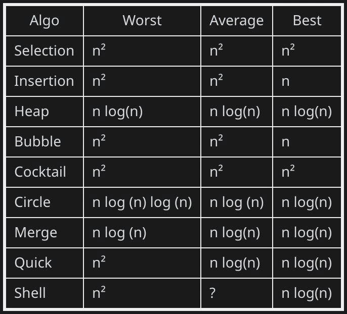
A Developer's Sorting Algorithm Cheat Sheet

Level 1: Sorting Socks

Imagine you have a big pile of socks of different colors and you want to sort them (say, pair them up or arrange by color). You have a bunch of different strategies to choose from, just like these different sorting algorithms. The chart in the meme is basically telling us how long each strategy might take in different scenarios – kind of like race times for each strategy. Let’s put it in very simple, everyday terms:

• Selection sort is like sorting the socks by always looking through the whole pile to find the next sock in order. Say you want to sort by color; you’d scan the entire pile to find the next red sock, put it in place, then scan the whole pile again to find the next, and so on. This method is very slow no matter what. Even if the socks were almost sorted already, you’d still stubbornly scan through all of them every time to make sure you’re picking the right one. It’s thorough, but it wastes a lot of effort. So in the chart, selection sort’s times are slow in the worst case, average case, and even the best case – it always takes a long time.

• Insertion sort is like sorting socks by taking one sock at a time from the pile and inserting it into a sorted drawer of socks. If the pile is already pretty organized (imagine the socks were almost all paired or arranged by color already), then each sock you pick up easily goes to the right spot without much shuffling – this would be really quick. But if the pile is completely messy (socks all jumbled in opposite colors), every time you pick a sock you might have to move a bunch of other socks in the drawer to insert it in the correct place – that gets really slow. So insertion sort can be fast if things are already in order (best case), but usually, with a random messy pile, it takes a lot of work (average case), and in the worst mess, it’s as slow as our first method.

• Heap sort is like having a special basket that always lets you grab the smallest sock (say, the next sock in alphabetical color order) quickly from the pile. Imagine you have a magic basket: you toss all your socks in it, and it somehow keeps them arranged such that you can always pluck out the next sorted sock in a snap. Using this basket (which is like a heap data structure), you ensure that grabbing the next item is efficient. No matter how the pile was to start, this method will take about the same amount of time relative to the size of the pile. It might not be the absolutely fastest for every single situation, but it’s consistently good. In the chart, heap sort’s times are the same for best, average, worst – always fairly fast for large piles.

• Bubble sort is like sorting socks by repeatedly going through the pile and swapping any two socks that are in the wrong order. Imagine you go through the pile comparing adjacent socks and if a blue sock comes before a red sock and you want red first, you swap them. You keep doing this again and again, multiple passes, until no socks are out of order. If the pile is very jumbled, you’ll be doing a ton of swapping passes, which is very slow (that’s the worst case). If the pile was actually already sorted to begin with, you’d go through once, find nothing to swap, and be done – that’s quick (best case). So bubble sort can detect a sorted pile fast, but if the pile is random, it’s going to take a long time because it keeps bubbling things into place slowly.

• Cocktail sort is a slight variation of the above: it’s like bubble sort but you go left-to-right then right-to-left in the pile, back and forth, swapping out-of-order socks both ways. It’s as if you first walk through the pile pushing the largest socks to the end, then you walk backwards through the pile pushing the smallest socks to the beginning, and repeat. It sounds fancy, like doing a little dance through the pile, but in reality it doesn’t speed things up much. It will still take a long time for a messy pile, about the same as bubble sort. So, its times are about as slow as bubble sort in most cases.

• Circle sort is a quirkier strategy. Imagine if you spread your socks in a line and then repeatedly compare socks that are far apart, like the one from the left end with one from the right end, swapping them if they’re out of order, then moving inward (like comparing socks in pairs from opposite ends, going toward the center). You do that pairing and swapping, then you recursively do it on smaller sections of the line. It’s like sorting the outermost pairs, then the inner pairs, and so forth. This method is a bit odd – it usually sorts the pile in a reasonably fast time, but in the worst case (some kind of particularly unlucky initial arrangement) it might take somewhat longer (with that extra log factor in the formula, but we won’t worry about the exact meaning of $\log$ here – just “a bit more work”). Think of it as a strategy that’s generally efficient but has a somewhat unpredictable upper limit on time. It’s not as commonly used, it’s just a creative way to pair up socks from ends towards the middle.

• Merge sort is like organizing the socks by first splitting the pile into two smaller piles, sorting each of those piles, and then carefully merging the two sorted piles back together. You keep splitting piles into halves until you have lots of tiny sorted piles (sorting two socks or one sock is trivial), and then you merge them step by step. For example, split your big pile into two, sort those; to sort each half you might split into quarters, and so on. Merging two sorted piles is efficient: you just repeatedly take the smallest sock from the front of either pile and build a new combined sorted pile. This divide-and-conquer approach is very efficient and consistent. No matter how the socks were initially mixed up, you’re always going to do about the same amount of work relative to n. There’s no particular worst-case scenario that’s worse than average for merge sort – even a terribly mixed pile sorts in pretty much the same time as an average mixed pile. So merge sort is reliably good (that’s why the chart shows the same time complexity for all cases). The trade-off is that while merging, you might need some extra space (like a spare table to lay out socks while merging two piles), but time-wise it’s on point.

• Quick sort is like sorting socks by picking one sock as a “pivot” (say you grab a random sock) and then splitting the pile into two piles: one with all the socks that should come before that pivot sock in order, and one with all that should come after. Then you sort those two piles in the same way (each time picking a pivot in a pile and splitting). Finally, you combine them together (actually, in quick sort you don’t explicitly combine like merge sort; the dividing process by pivots ultimately produces a sorted order in place). Now, if you pick a good pivot each time – roughly a sock that’s medium, so the piles are about half-half – then you’re golden: the pile size shrinks quickly and the sorting goes fast (that’s the average case and best case scenario). But if you’re really unlucky and each time you pick, say, the smallest sock as pivot (so one pile is of size n-1 and the other is 0 – basically not splitting at all properly), then you’re doing all the work of splitting but not reducing the problem much each time. That leads to taking much longer – that’s the dreaded worst case. In human terms, it’s like if your strategy for sorting socks sometimes leads you to make very uneven groups and you have to sort almost the whole thing again and again. Usually quick sort is very fast (it’s one of the fastest in practice on average), but we keep in mind that in theory it can misbehave if you always somehow choose a terrible pivot. Many practical quick sort routines have ways to avoid the bad luck consistently. So on the chart, Quick sort has two faces: mostly $n \log n$ (efficient) but worst-case $n^2$ (much slower) if you’re unlucky with those pivot choices.

• Shell sort is a bit like a multi-stage approach to sorting the socks. Think of it this way: you first roughly sort the socks by looking at socks that are far apart in the pile and sorting those, then you do it with smaller gaps, and then finally you do a last pass to fully sort them. In practice, imagine laying out socks in a row and first making sure every 10th sock is in order relative to the others in those positions, then every 5th sock, then every 1 (which is just a normal final pass). By doing those earlier gap-based sorts, the idea is the pile gets “more ordered” and by the end the last pass is quick. Shell sort was one of the first attempts to improve on insertion sort’s speed by doing this hopping. Now, how long Shell sort takes can vary a lot depending on how you choose those gap steps and also on the initial arrangement. It usually runs pretty fast (faster than bubble or insertion for medium-sized piles), but pinning an exact formula for its average time is tricky. That’s why the chart cheekily puts a "?" for Shell sort’s average time – it’s saying “we’re not quite sure, it’s complicated.” We do know worst-case could be as bad as $n^2$ if you’re unlucky with how the gaps work out or choose poor gaps. Best case might be around $n \log n$ (if the socks were almost sorted to start with or the gap sequence works out perfectly, it sorts quickly). But on average, people just know Shell sort is better than $n^2$ typically, but not as good as $n \log n$ of the really fast sorts. So it sits in a kind of grey zone, and the chart just leaves it at that with a shrug (the "?").

Why is this table funny or interesting in simple terms? Well, it’s like making a little scoreboard for different ways to do the same chore (sorting socks, or any collection). Some methods are always slow, some are usually fast but can be slow if you're unlucky, some are steady and reliable, and one is like “we’re not even sure how to rate it!” Seeing that one method just has a question mark for the average case is a bit like having a friend whose speed at cleaning their room is totally unpredictable – it might be really fast one day and slow the next, so you just put a “?” in their scorecard. For someone learning this stuff, the chart is a quick way to remember each method’s personality. And the little joke is that Shell sort is so quirky that even in a serious summary, we throw up our hands and say "Who knows?"

So, in everyday analogy: imagine lining up nine different people each with their own strategy to sort the same messy pile of socks. Eight of them you can kind of predict:

• Some will always take forever (the meticulous one who checks every sock every time, like selection sort).
• Some will usually do okay and sometimes zoom through if the socks were already sorted (the one who goes with the flow if things are easy, like insertion sort).
• Some are consistently efficient, methodical sorters (the two who split tasks or use special tools, like merge sort and heap sort, always performing well).
• One is usually super quick but if he picks the wrong starting sock, oh boy, he gets stuck reorganizing way too much (the quick sorter).
• One person tries a funky back-and-forth approach (cocktail) which looks cool but doesn’t really save time.
• Another does the weird opposite-ends-at-once strategy (circle sort), usually fine but occasionally it doesn’t help much if the socks are arranged in a particularly troublesome way.
• And then there’s that one person with the multi-step quirky method (shell sort) – most of us just watch and go “I think it works most of the time?”

The meme is a reminder of all these strategies and their efficiencies. It’s kind of amusing because it takes something that can be very mathy (Big O notation and algorithms) and boils it down to a simple table – which ends up looking like a little scoreboard of sorting races. If you’re new to this, the key thing to get is: not all sorting methods are equal; some are a lot faster than others, especially as the number of items grows. And the chart is a quick cheat-sheet of who wins the race most of the time (the ones with $n \log n$) and who falls behind (the ones with $n^2$), with one or two special notes (like the question mark) for the oddballs. It’s both educational and a bit playful, making the world of sorting algorithms a tad more approachable at a glance.

Level 2: Sorting Out Sorting

Let’s break down what this chart is showing in a more beginner-friendly way. This meme is essentially a quick reference table comparing the running time of nine different sorting algorithms. When we talk about running time in computer science, we often use Big O notation to describe how the time grows as the number of items (n) grows. The table has three columns for each algorithm: Worst case, Average case, and Best case. These refer to how the algorithm performs under different conditions:

• Worst case: This is when the input is arranged in the most unfavorable way for the algorithm, causing it to take the longest time.
• Average case: This is the typical running time you’d expect for a random order of input.
• Best case: This is when the input is arranged in the most favorable way (often nearly sorted), and the algorithm runs fastest.

The entries like $n^2$ or $n \log(n)$ are the Big O notation describing the time complexity. Here, n usually means the number of elements being sorted. So:

• $n^2$ (spoken as “n squared”) means the time grows proportional to the square of the number of elements. If you double the number of elements, the work might roughly quadruple. That’s quite slow for large n.
• $n \log(n)$ (spoken “n log n”) means the time grows proportional to n times the logarithm of n. This grows faster than linear ($n$) but much slower than $n^2$. For example, if n doubles, $n \log n$ maybe roughly doubles a bit more (since log n grows slowly).
• $n$ means linear time – if the number of items doubles, the work doubles (this is pretty efficient).
• A question mark “?” here humorously indicates uncertainty or complexity that’s not easily expressed – meaning we don’t have a simple formula for that case.

Now, let’s briefly explain each sorting algorithm and why their entries in the table are what they are:

• Selection Sort: This algorithm selects the smallest (or largest) element from the unsorted portion and moves it to the sorted portion, one element at a time. Imagine sorting a stack of cards by always looking through the whole stack to find the next smallest card to put in order. No matter how the cards are arranged to start, selection sort will still look through everything to find the next item each time. That’s why its best, average, and worst cases are all $O(n^2)$. It always does roughly the same number of comparisons (about $\frac{n(n-1)}{2}$ comparisons in total) regardless of input order. So in the table, Selection sort shows n² for Worst, n² for Average, n² for Best.

• Insertion Sort: This one builds the sorted list one item at a time by inserting each new element into the correct position among the already sorted ones (like the way many people arrange playing cards in their hand). If the input list is already almost sorted, insertion sort has very little to do – each new element is already in the right spot or maybe needs just one swap, so that’s why the best case is $O(n)$ (pretty much just one pass through the list without much shifting). However, if the list is in the worst possible order (for insertion sort, that’s usually reverse sorted, because every new element has to be moved all the way to the front), it will end up doing a lot of comparisons and moves – roughly on the order of $n^2/2$ operations, which simplifies to $O(n^2)$. The average random order also yields about $O(n^2)$ steps. So the table shows: Worst n², Average n², Best n. In short, insertion sort is great for nearly sorted data (linear time) but can be slow (quadratic time) in general.

• Heap Sort: Heap sort uses a heap data structure (often a binary heap, which can be visualized as a kind of tree or as an array where you can efficiently get the largest or smallest element). The process is: build a heap out of all elements (which takes $O(n)$ time for a heapify operation), then repeatedly remove the largest element from the heap and put it into the sorted portion. Removing from a heap or inserting into a heap takes $O(\log n)$ time, and you do it n times, so that’s $n \times \log n$. Therefore, heap sort’s worst, average, and best cases are all $O(n \log n)$. It doesn’t matter what the initial order of the elements is – using the heap structure guarantees that upper bound on time. In the table we see Heap: n log(n), n log(n), n log(n). This consistency is a big advantage of heap sort: it’s reliably efficient in any case (though one downside is it might not be as cache-friendly as some others, but that’s another story).

• Bubble Sort: This is the classic simple sort where you repeatedly go through the list, compare each pair of adjacent items, and swap them if they’re in the wrong order. It’s called bubble sort because each pass “bubbles up” the largest element to the end of the list (like bubbles rising to the surface). Bubble sort is very slow in general – if the list is in random order, you might have to pass through the list about n times, and during each pass you do roughly n comparisons/swaps, yielding about $n \times n = n^2$ operations (worst and average case $O(n^2)$). However, bubble sort has a nice property: if the list becomes sorted early, it can stop. In the best case scenario (which is when the list is already sorted to begin with), the algorithm will go through once, find no swaps needed, and stop immediately. That’s one pass of ~n comparisons, making it $O(n)$ for best case. So in the table, Bubble sort is n² for Worst, n² for Average, and n for Best. In other words, normally quadratic time, but it can recognize a sorted list quickly. Still, it’s generally not efficient for large n.

• Cocktail Sort: Also known as shaker sort, this is basically a slight twist on bubble sort. Instead of only going one direction (left to right) each pass, cocktail sort goes both directions: left-to-right doing swaps, then right-to-left doing swaps, in a back-and-forth fashion per full cycle. The idea is to bubble up largest items to the right and bubble down smallest items to the left in each pair of passes, potentially sorting slightly faster than standard bubble sort in some scenarios. However, in terms of Big O complexity, it doesn’t actually improve things fundamentally. It still compares adjacent items and still might have to do multiple passes if the list is unordered. So it ends up being $O(n^2)$ in the worst case and on average as well. Depending on implementation, its best case might also be $O(n)$ if it checks and finds the list sorted (much like bubble sort does). The table given shows Cocktail sort as n², n², n² (so perhaps assuming a version that doesn’t short-circuit early, or just emphasizing it’s usually $n^2$). The key takeaway: cocktail sort is basically bubble sort with a twist, but it’s not fundamentally faster in big picture terms.

• Circle Sort: This one might be new if you’re just learning fundamentals – it’s not typically covered in intro classes. Circle sort is a more unusual algorithm. The basic concept is to recursively sort the list by comparing and swapping items that are positioned at equal distance from the ends, kind of “around” the list (like first and last, second and second-last, etc., treating the list like a circle). After one full pass, it recurses on smaller sections (like halving the problem and doing it again on each half). The complexities given in the table (Worst: n log(n) log(n), Average: n log(n), Best: n log(n)) show that circle sort tends to run in about $O(n \log n)$ on average and best conditions (so it’s comparable to the faster algorithms), but in the worst case it has an extra $\log n$ factor (so $O(n (\log n)^2)$). That means if you give it a particularly troublesome input, its dividing strategy might not work perfectly and it ends up doing somewhat more work than the optimal algorithms. Still, $n (\log n)^2$ is better than $n^2$ for large n (for example, if n = 1000, $\log_2(1000)\approx10$, so $n(\log n)^2$ ~ 1000*100 = 100k, versus $n^2$ which is 1,000,000). Circle sort is mostly included here for completeness or curiosity – it’s not commonly used in everyday programming, but it’s a neat variation in the algorithm design space. The table listing it is likely to spice up the comparison and show that not all sorting algorithms fit the basic mold.

• Merge Sort: A very important and popular sorting algorithm, merge sort uses a divide-and-conquer approach. It splits the list into two halves, sorts each half (recursively, using merge sort), and then merges the sorted halves together. Merging two sorted halves takes linear time $O(n)$ (since you just compare the front elements of each half and keep taking the smaller one). The splitting happens about $\log_2 n$ levels deep (since you keep halving the list until you get down to single elements). So the total work is roughly $O(n)$ merge per level times $\log n$ levels = $O(n \log n)$. Merge sort’s behavior doesn’t really depend on the initial order of the data – it will always do the same number of comparisons and merges regardless. Thus, its worst, average, and best are all $O(n \log n)$. The table shows that consistency. This reliability is why merge sort is often taught as a gold-standard sorting method. One thing to note: merge sort requires extra memory space for the merging process (to hold temporary arrays), but in terms of time, it’s steadily efficient. Many programming languages use variants of merge sort (like Timsort in Python, which is a hybrid but based on merge sort) for their default sorting because it’s predictable and stable (maintains order of equal elements).

• Quick Sort: Quick sort is another divide-and-conquer algorithm, but it works quite differently from merge sort. Quick sort picks a “pivot” element and partitions the list into two groups: items less than the pivot go on one side, items greater go on the other side. Then it recursively sorts the two groups. The idea is that if the pivot chosen is reasonably in the middle, the two groups are about half the size of the original, and the recursion depth is $\log n$ (like merge sort). The partitioning step itself is $O(n)$ (you inspect each element and compare to the pivot to divide them). So in the ideal scenario, you again get $O(n)$ work per level times $\log n$ levels, which is $O(n \log n)$. That’s why the average complexity is $O(n \log n)$; with a random pivot or random input, you’re likely to get reasonably balanced splits. The best case is also $O(n \log n)$ (that’s if you always pick the perfect pivot each time – e.g., the median – then halves every time). However, the worst case is $O(n^2)$. Worst-case happens when the pivots are chosen poorly so that one of the partitions has almost all the elements and the other has almost none. For example, if you always choose the last element as pivot and the array is already sorted in increasing order, each partition step might only peel off one element, leaving n-1 on the other side. That makes the recursion depth n (instead of log n), and you end up doing roughly $n + (n-1) + ... + 1$ comparisons, which is about $n^2/2$. Many quick sort implementations guard against this by choosing a random pivot or using techniques like “median-of-three” (pick the median of first, middle, last as pivot) to avoid always hitting the bad case. There’s even Introsort (used in C++ STL) which switches to heap sort if it detects too many levels of recursion (to cap the worst-case). The table’s Quick sort row (Worst n², Average n log(n), Best n log(n)) is a straightforward reminder of this dual nature. This is arguably the most critical entry in such charts during interviews – people often ask “What’s Quick sort’s complexity?” expecting you to remember both typical and worst cases.

• Shell Sort: Shell sort is like an optimized version of insertion sort. It works by comparing and swapping items that are far apart to begin with (using a gap), then reducing the gap size gradually until in the final step, it’s doing regular insertion sort (gap of 1). The idea is that by the time you get to that final pass, the list is “mostly sorted” so insertion sort can finish it quickly. The tricky part is, Shell sort’s performance is very sensitive to how you choose the gap sequence (the series of gap values you use). Different sequences yield different results, and analyzing it mathematically gets complicated. Many sequences have been proposed (Shell’s original sequence, Hibbard’s, Knuth’s, Pratt’s, etc.), each affecting the running time. For many practical sequences, the worst-case might be $O(n^2)$ (like if gaps aren’t well chosen). Some sequences give better worst-case bounds (like $O(n^{3/2})$ or other strange expressions). Empirically, Shell sort runs quite fast on average for medium-sized arrays, but theoretically deriving its average-case complexity is hard. That's why in the cheat sheet, the Average column for Shell sort is just “?”. It means we can’t easily summarize it with a simple formula – it’s not a neat $n^2$ or $n \log n$. It depends. We do know the best case for Shell sort can be as good as $O(n \log n)$ (for example, if the data is already sorted, Shell sort will just do a few passes and find nothing much to swap, similar to insertion sort's best case). The worst case listed is $n^2$, likely assuming a common gap sequence where that’s true. But overall, Shell sort lands somewhere between linear and quadratic time on average; for good gap sequences it might be around $O(n^{1.25}$ to $O(n^{1.5})$ in practice). The question mark is a playful way to say “average case is complicated.” This reflects a bit of reality: even computer scientists sometimes say "Shell sort’s average complexity: we think it's about this range, but it’s not as clean-cut."

So, the table is summarizing time complexity which is a measure of performance in terms of how the algorithm’s running time grows with input size. It’s a key part of CS fundamentals and Algorithm Complexity Analysis to know these. For a newcomer, you can interpret this cheat sheet like so:

• If you see $n^2$ vs $n \log n$, understand that $n^2$ grows much faster. For instance, if you have 1000 items, $n^2` means roughly 1,000,000 steps, while $n \log n$ is roughly 1000 * 10 = 10,000 steps (since $\log_2(1000)\approx10$). That's a huge difference!
• Algorithms with $n^2$ are generally considered inefficient on large data sets (they might be fine for small n, like n=50 or 100, but they’ll bog down quickly as n grows).
• Algorithms with $n \log n$ are much more scalable to large inputs – they’re the ones you use for serious sorting of big lists.
• The best/average/worst distinction is important: some algorithms (like Quick sort) are usually fast but can have rare slow cases, others (like Merge sort) are steady, others (like Insertion sort) can be fast if you’re lucky (input nearly sorted) but usually slower as n grows.

Finally, the “Reminder” caption suggests this is a chart meant to remind us of these basics, possibly for quick recall. In programming discussions or interviews (tagged with things like SortingAlgorithms and AlgorithmDesign), these are go-to facts. Each algorithm name listed (selection_sort, insertion_sort, etc.) is like part of the vocabulary of classic algorithms. This meme conveniently lines them up so you can compare their efficiency side by side.

In summary, this cheat sheet is saying: Here’s a quick at-a-glance comparison of how nine different sorting methods scale. For someone learning, it’s a handy chart to memorize or understand. And it even sneaks in a bit of nuance (with Shell sort’s uncertainty and the inclusion of a quirky one like Circle sort) to remind us that not everything is black-and-white, but most of the common algorithms can be neatly described with these Big O terms. Understanding this table is a fundamental step in grasping algorithm performance – it’s the kind of knowledge that sticks with you throughout your programming journey.

Level 3: Sorting Showdown

For a seasoned developer or anyone who’s been through the crucible of a coding interview or a CS algorithms class, this image hits like a flashback. It’s basically the Big-O cheat sheet for common sorting algorithms – the kind of table you might scribble on a whiteboard while cramming for an exam or prepping for whiteboard interviews. The meme’s caption "Reminder" suggests that it’s meant to jog our memory: “Hey, remember your sorting complexities? Here they are at a glance.” And sure enough, experienced folks will glance at this and mentally tick off each row: Selection sort? Yep, always $n^2$. Quick sort? Average $n \log n$ but watch out for the $n^2$ worst-case. It’s almost comforting in a nerdy way – like seeing old familiar friends (or rivals) line up for a race and knowing exactly how they perform.

The humor or delight here comes from recognition and a bit of “insider” perspective. For one, the algorithms are listed sort of like contestants in a performance contest, with their Worst, Average, and Best cases as stats. If you’ve been around the block, you know this stuff cold (or at least you’re supposed to, whenever a tough interview question comes up). Seeing it laid out so neatly is oddly satisfying. It’s like those sportscards with player stats, but for algorithms – and any developer who’s had to optimize a sorting routine or answer “Why is quicksort usually faster than mergesort?” will appreciate having these stats at the ready.

Let’s talk about the contestants in this sorting showdown, and why they make us smirk:

• Selection Sort is the slow-but-simple one. You can almost hear the collective groan: $O(n^2)$ across the board (worst, average, best). This algorithm is the embodiment of “no matter what you do, I’m gonna take my sweet time.” Even if the data is already sorted, selection sort still grinds through every comparison. Experienced devs joke that selection sort is basically the algorithmic equivalent of checking every single book on a shelf one by one to find the smallest, and doing that for each position on the shelf – thorough but super inefficient. The meme lists $n^2, n^2, n^2$ almost in a deadpan way: consistent, but consistently bad. It’s a gentle jab at how un-optimized this method is. In real life, you’d rarely use selection sort except maybe for teaching purposes or very small datasets.

• Insertion Sort and Bubble Sort – these two share a similar $O(n^2)$ fate in the average and worst cases, but they have a redeeming quality: best-case $O(n)$. The table highlights that contrast: average $n^2$, best $n$. For those in the know, this immediately says “We can detect sorted data!” Both of these algorithms can finish early if the list is already sorted or nearly sorted. Bubble sort will do one pass and realize nothing needs swapping; insertion sort will keep inserting elements that are already in the correct position with just one comparison each. For a developer, this is a hint: these algorithms are adaptive to good cases. There’s a bit of humor seeing $n$ in the best column – it’s like saying, “Hey, I’m not always slow!” An experienced dev might chuckle because they remember that one time they told someone, “Bubble sort is $O(n^2)$... well, unless your data is already sorted, in which case it’s like, instant.” It’s the classic caveat we attach when we don’t want to unfairly malign an algorithm. But still, nobody in their right mind uses bubble sort for large data – that $n^2$ average is a killer. The meme silently affirms that: in the average column it’s $n^2$, meaning typically, yeah, it’s slow.

• Heap Sort and Merge Sort are the solid performers – $O(n \log n)$ consistently. The table’s symmetry for these (same $n \log n$ in worst, average, best) is oddly pleasing. Any senior dev glancing at that goes, “Mm-hmm, the workhorses.” It’s a reminder why these algorithms are taught as good general-purpose sorts: they don’t have a surprise bad case that blows up on you. In practice, you often won’t implement these by hand (you rely on library functions), but you know under the hood Python’s sorted() might be Timsort (derived from merge sort) or C++ std::sort might be Introsort (quick sort + heap sort fallback). Either way, those guaranteed $n \log n$ algorithms are in there to ensure things stay efficient even in edge cases. A knowing smile might come from noticing Heap sort in the list – it’s famously not used as often in practice as Quick sort or Merge sort (due to cache behavior and constant factors), but as an experienced dev you respect it as the worst-case insurance sort. That $n \log n$ in the Worst column is like a safety badge.

• Quick Sort is the star of many coding interviews, and the table doesn’t disappoint: it shows the classic algorithmic trade-off. Seeing $n^2$ in the Worst column and $n \log n$ in the Average/Best columns instantly paints the picture of Quick sort’s nature. An experienced engineer likely recalls the war stories: “We got hit by Quick sort’s worst-case once when our input was already sorted and our naive implementation kept picking the first element as pivot—boy, did that tank performance!” It’s almost a rite of passage to learn why Quick sort, despite that scary $n^2$ worst-case, is usually okay (randomize those pivots, or use median-of-three). The dual personality of Quick sort is a great conversation piece: it’s usually excellent, but you have to be aware of that Murphy’s Law scenario where it degenerates. The meme’s succinct presentation of that is kind of funny because it’s so stark: as if Quick sort is an honor student with a not-so-secret dark side. For seasoned devs, it’s a reminder that average-case matters a lot in real life, and why Quick sort is beloved (fast average) yet why we design safeguards (to avoid the rare worst-case).

• Cocktail Sort being listed might draw a chuckle or raised eyebrow from experienced folks. Cocktail sort (aka shaker sort) is basically a variant of bubble sort that goes both left-to-right and right-to-left in each pair of passes. The meme shows $n^2$ for worst, $n^2$ for average, and $n^2$ for best as well (assuming the table says the same for Cocktail as selection? Actually, the table says Cocktail – n², n², n²). Wait, did it list best-case also $n^2$ for cocktail? The description above lists "Cocktail – n², n², n²" which implies even best-case is $n^2$. If that’s accurate (often cocktail sort best-case is also $O(n)$ if you break when no swaps made, though maybe the simplest implementation doesn’t break early in both directions?). If it’s indeed n² across the board in the meme, that’s a tongue-in-cheek jab: it means this “fancy-sounding” bubble variant offers no asymptotic improvement at all. As a senior dev, you smirk at that because it reaffirms a truth in software engineering: a fancy name doesn’t guarantee better performance. It’s almost sarcastic: “You can shake the list back and forth like a cocktail shaker, but guess what – you’re still in the $n^2$ club!” So cocktail sort is basically bubble sort’s flamboyant cousin who, despite doing a little dance in both directions, ends up with the same complexity. It’s a light reminder that many such variants exist and they don't change the Big O, which is a very “we’ve seen it all” veteran perspective.

• Circle Sort being on this list definitely falls into the “flexing obscure knowledge” category. A lot of experienced devs might go, “Oh yeah, circle sort…I’ve heard of that… I think.” It’s not common in everyday work or interviews, so its presence is half educational, half humorous. The values given (worst $n \log(n)\log(n)$, average $n \log(n)$, best $n \log(n)$) might make the reader grin and think, “Whoa, that worst-case is funky!” It’s not every day you see $n \log n \log n$ in a complexity chart. Reading that out loud feels like a tongue-twister: “en log en log en.” It almost looks like a mistake or a stutter, which might be part of the meme humor – double logs aren’t typical in the basic sorting algorithm roster. For the seasoned crowd, it’s a reminder that there are all sorts of strange sorting algorithms concocted in academia or recreational programming. Maybe someone recalls reading about circle sort in a blog or watching a visual sorting demo on YouTube. The fact it’s included here is a bit of a wink: “We’re not just covering the usual suspects; we’ve got some remix versions too.”

• Finally, Shell Sort with its notorious question mark “?” in the Average column is definitely an inside joke for those who know their algorithm basics. It’s like the chart is saying, “Average case for Shell sort? Your guess is as good as mine!” Of course, in reality, computer scientists have studied Shell sort, but the humor is that unlike the neat $n^2$ or $n \log n$ of others, Shell sort’s complexity analysis is messy. Any experienced dev who took Algorithms 101 remembers that Shell sort was this oddball: it’s faster than insertion sort in practice, but giving a single clean Big-O for it is tricky. Seeing the question mark in a polished cheat-sheet is funny because cheat-sheets are supposed to have all the answers, yet here the creator just throws up their hands for Shell sort. It almost personifies Shell sort as the enigmatic one among the group — “Shell sort, what are you on average? Eh, it’s complicated.” If you’ve been around, you appreciate that honesty. Perhaps you recall that Shell sort’s complexity can range widely with different gap sequences, or that it’s subject of academic analysis. The question mark is both a small joke and a truth: ask five algorithm gurus about Shell sort’s average complexity and you’ll get a lot of hemming and hawing or conditional answers. So in a list meant as a quick “reminder,” leaving a "?" is ironically relatable.

Overall, the meme functions as a quick performance comparison chart, and a seasoned viewer finds it engaging because it condenses so much knowledge into a tiny table. The experienced perspective also notes what’s not said: real-world performance isn’t only about Big-O. Constants, memory usage, data distribution, and usage patterns matter. But for a high-level discussion or interview, Big-O is the language everyone speaks. This table is basically the lingua franca of performance for sorting: it’s how we communicate which algorithm is generally faster or slower.

The fact that it’s an image (with that slick dark background and bright text) also tickles the inner nerd: it’s like a cheat-sheet aesthetic, something you might tape to a wall or save on your phone for quick reference. It triggers the memory of study guides or those “big O notation” posters. When the post says "Reminder", an experienced dev might grin and think, “Yep, I remember spending nights memorizing that exact info.” It could also be seen as a tongue-in-cheek reminder that not all sorting algorithms are created equal, so choose wisely.

In daily developer life, you rarely implement these from scratch (most languages have highly optimized library sorts), but knowing their differences is crucial in debugging performance issues or understanding why a sort operation is slow. So this meme serves as both a nostalgic nod and a practical refresher. It’s the kind of thing you tag a junior colleague in and say “Here’s that chart you asked for,” or you share in a dev forum to spark a round of “Haha, Shell sort…amirite?” banter. It’s funny in a nerdy way, and useful – a perfect mix for the programmer humor world.

Level 4: The Logarithmic Limit

In the realm of algorithm analysis, sorting is a classic battlefield where mathematics meets code. At the deepest theoretical level, this meme’s table is hinting at the fundamental limits of sorting by comparisons. There’s a well-known result in computer science that any general-purpose sorting algorithm based solely on comparing elements has a theoretical lower bound of $O(n \log n)$ in the worst case. This comes from an information-theoretic argument (imagine a decision tree of comparisons; sorting $n$ items has $n!$ possible outcomes, and the tree must have depth at least $\log_2(n!) = O(n \log n)$ to distinguish all permutations). In simple terms, you can’t sort faster than proportional to $n \log n$ time on average if all you do is compare elements, because that’s the minimum number of yes/no decisions needed to pinpoint the correct order.

Now, notice how several algorithms in the chart bump right against this logarithmic limit. Algorithms like Merge sort and Heap sort proudly show $O(n \log n)$ for worst, average, and best cases. They are the optimal comparisons sorts in terms of order-of-growth – they always operate within a factor of $n \log n$. These algorithms achieve the theoretical limit by very different means: Merge sort uses a classic divide-and-conquer approach (splitting the array and merging sorted halves with linear merging cost $O(n)$ at each level, across $\log n$ levels of recursion). Heap sort uses a binary heap data structure to always extract the next smallest element in $O(\log n)$ time, doing that $n$ times for $n \log n$ total. They exemplify how careful algorithm design hits the $n \log n$ wall in both theory and practice.

On the flip side, some algorithms in the table fall short of this optimal limit, and theory tells us they pay a price in asymptotic performance. Selection sort, Bubble sort, Insertion sort, and Cocktail sort all have $\bold{O(n^2)}$ worst-case behavior, well above the $n \log n$ lower bound. That means in the worst scenario (and for some of them, even on average) these methods perform quadratic work — the time grows proportional to the square of the number of items. Why such a high order? It’s because these simpler methods don’t effectively reduce the problem’s decision complexity; they end up making on the order of $n^2$ comparisons or swaps in the worst case. For example, Selection sort naively picks the smallest remaining element by scanning the entire list for each of the $n$ positions (leading to roughly $n + (n-1) + ... + 1 \approx n^2/2$ comparisons always). No matter how sorted the input already is, selection sort stubbornly does the full scan for each element – hence its best, average, and worst cases are all $O(n^2)$. It completely ignores any existing order in the data, which from an information perspective means it’s doing a lot of redundant work.

Contrast that with Insertion sort or Bubble sort, where the best-case is $O(n)$. Those algorithms are able to exploit an input that’s already sorted or almost sorted. The meme’s table highlights this by showing a best-case of $n$ (linear time) for Insertion and Bubble. In theoretical terms, these algorithms have adaptive complexity: if the data is easy (like sorted), they finish faster. Why? In insertion sort, if the list is already sorted, each new element is just compared once with its immediate predecessor and placed – no shifting needed – giving linear performance. In bubble sort, if no swaps are needed during a pass (i.e., the list is sorted), the algorithm can terminate early after one pass. However, their average and worst-case still degrade to $O(n^2)$ for random or adversarial data, meaning they still ultimately break the $n \log n$ barrier in a bad way when $n$ grows large. From a theoretical lens, insertion and bubble sort have best-case linear time because they can detect sorted order quickly, but in the average case they end up examining many inversions (out-of-order pairs), which for random data is on the order of $n^2$ pairs in expectation.

Then there’s Quick sort, an algorithm that teases the optimal $O(n \log n)$ behavior on average but can betray us in the worst case. The table shows Quick sort as Worst: $n^2$, Average: $n \log(n)$, Best: $n \log(n)$. This dichotomy is a classic result from average-case analysis: Quick sort’s expected running time is $O(n \log n)$ (assuming all permutations of input are equally likely or pivots are chosen randomly). Mathematically, one can derive this by solving a recurrence relation for the average cost or integrating over all possible pivot positions; it turns out to involve a harmonic series that simplifies to a linearithmic order. But if you feed Quick sort pathological input or consistently pick poor pivots (like always choosing the first element as pivot when the array is already sorted), it degrades to $O(n^2)$. The reason is that those unlucky pivot choices produce extremely unbalanced partitions (one side of the split has almost all elements and the other side has very few). In decision tree terms, Quick sort’s worst-case recursion tree becomes basically a chain of $n$ levels with $O(n)$ work at each level, hence $O(n^2)$. The theoretical insight is that Quick sort doesn’t guarantee balanced partitions unless randomization or median-of-three pivot strategies are used. Introsort (used in some standard libraries) cleverly mitigates this by switching to Heap sort if recursion goes too deep, ensuring $O(n \log n)$ worst-case – a practical blend of algorithms to respect the $n \log n$ limit.

Now, a very intriguing part of this meme is the inclusion of Shell sort and Circle sort, which venture into less-charted territory of analysis. The table cheekily puts a "?" for Shell sort’s average complexity – a nod to the fact that Shell sort’s average-case complexity is notoriously hard to pin down. Shell sort (invented by Donald Shell in 1959) is essentially a generalization of insertion sort that gains speed by hopping elements long distances early on (using gap intervals that shrink over time). Its exact running time depends heavily on the chosen sequence of gaps (increments). The worst-case of Shell sort is often $O(n^2)$ for many simple gap sequences (like Shell’s original sequence or others), but some gap sequences can improve the worst-case. It’s known from deeper algorithmic research that a good gap sequence (like Pratt’s sequence or Ciura’s empirically derived gaps) can yield better performance; some specific sequences have been conjectured or proven to give worst-case bounds like $O(n^{3/2})$ or $O(n \log^2 n)$. However, a general closed-form expression for Shell sort’s average-case complexity remains elusive in analytic combinatorics. In fact, as of the meme’s date and even today, the exact average-case complexity of Shell sort for the best known gap sequences isn’t a simple $n^p$ or $n \log n$ form – hence the cheeky ‘?’ in the table. It’s a playful acknowledgement among CS folks that even after decades of study, Shell sort keeps some secrets. The question mark is academically honest (since average-case analysis can be extremely complex) and also a bit humorous – it’s like saying “don’t ask, it’s complicated.”

Circle sort is another intriguing entry. The table lists Circle sort’s worst-case as $n \log(n) \log(n)$ – which basically means $O(n (\log n)^2)$. This is an unusual complexity and likely indicates that Circle sort isn’t hitting the ideal $O(n \log n)$ boundary but is still better than quadratic time. Circle sort is a less common algorithm (you won’t usually find it in standard textbooks), but it’s known among algorithm enthusiasts as an interesting recursive comparison sort. The idea behind Circle sort is to recursively pair up elements mirroring across the array (like first with last, second with second-last, and so on in a “circle”) and swap those that are out of order, then recursively sort the halves. It’s somewhat reminiscent of bitonic sort or other recursive partnering sorts. The double logarithm factor in its complexity suggests that each level of recursion does O(n) work (comparing and swapping pairs in one pass), and the recursion depth is $O(\log n)$ (like many divide-and-conquer sorts), but perhaps due to the nature of splitting (it might split into more than two parts or overlaps slightly), it introduces another $\log n$ factor in the number of levels. So maybe it's $O(n \log n)$ average with an extra log factor in the worst case due to some imbalanced recursion pattern. The specifics can get quite mathematical, but the key is: Circle sort doesn’t achieve the pure linearithmic ideal in the worst case – it’s a tad slower by that logarithmic factor, which places it in an intermediate complexity class between $O(n \log n)$ and $O(n^2)$. The presence of Circle sort in the table is almost certainly meant to flex some algorithmic trivia. It’s like saying, "we’re not just covering the basics, here’s an exotic one too!" It also highlights how diverse sorting methods can get, each with their own complexity behavior that theoretical computer science tries to characterize.

Finally, when looking at this chart from a theoretical altitude, one might also recall non-comparison sorts which are absent here. Algorithms like Counting sort or Radix sort can achieve linear time $O(n)$ or $O(nk)$ (for Radix with $k$ digit length) in certain scenarios by exploiting more information than just comparisons (they use the structure of keys, such as integer digit positions). Those escape the $O(n \log n)$ comparison barrier by not treating the data as arbitrary indistinguishable items – but such algorithms require assumptions (like a fixed range of numbers or treat keys in parts) and wouldn’t be included in a generic Big-O cheat sheet for comparison sorts. The meme stays within the classic comparison-based algorithms, which makes sense for a fair side-by-side. In summary at this deep level: this meme condenses a wealth of algorithmic complexity theory into a single image – reminding us of which sorting methods scrape against the theoretical best ($n \log n$) and which ones fall into the less efficient $n^2$ camp, and even admitting where our understanding (Shell sort’s average) isn’t neatly resolved. For seasoned algorithm enthusiasts, it’s both a handy reference and a tongue-in-cheek nod to the rich analysis behind those simple formulas.